This post is a follow-on from Part 1 which reported the experiences at the start of the heating season (at the end of November). After a few months of rather colder temperatures and the extraction of a considerable amount of heat from the ground, the Coefficient of Performance figures are still good but somewhat less impressive than before.

It’s evident that the temperature of the water coming in from the ground loop has a significant effect on the efficiency of the heat pump and the heat output it is able to deliver. At the end of November the ‘brine’ was typically coming in at 10 degrees whereas now it’s around 5 degrees. With brine at 10 degrees, the 8 kW heat pump was actually delivering 10 kW (as reported by the Kamstrup heat meter) whereas with brine at 5 degrees it’s ‘only’ delivering 8.5 kW. The heat pump experts tell me this is expected behaviour and it’s why an ‘open loop’ heat pump taking water from a lake or river performs better than a ‘closed loop’ unit which circulates the same brine around a closed circuit.

The headline performance statistics are now:

• In ‘heating’ mode, the unit is delivering an instantaneous CoP of around 4.25
• In ‘hot water’ mode, the unit is delivering an instantaneous CoP of as little as 2.75

Heating

In ‘heating’ mode the heat pump attempts to match the heat loss from the house by delivering water into the heating circuits at just the right average temperature. With colder temperatures outside this equates to warmer water, which tends to equate to lower efficiency (although actually the high thermal mass of the house reduces the impact of brief cold spells). During a typical ‘run’ it is still consuming almost exactly 2 kW (just like in November) but delivering 8.5 kW, for a CoP of around 4.25.

Hot Water

On cold-but-bright days, the hot water gets heated by the Immersun unit that diverts excess solar PV generation to the immersion heater, which has its thermostat set to 60 degrees. (It does this often enough that I’ve switched off the heat pump’s own anti-legionella sterilization cycle for the hot water tank.) On dull days the heat pump still kicks in to heat the stored hot water to 50 degrees. With the lower brine temperature (5 degrees in, 0 degrees out) it still consumes up to 2.88 kW but wth a reduced power output of 8.0 kW, for a CoP of 2.77.

Performance Graphs

The first set of graphs below are from a sample 24-hour period (2018-02-15T20:00 to 2018-02-16T20:00) which show:

• Some of the heat pump temperatures, as reported by its internal control system
• The heat pump power consumption, as reported by the sub-meter on its electricity input
• The heat pump power output, as reported by the heat meter on the ‘heating’ flow pipe from the heat pump

These graphs also show the ‘cycling’ of the heat pump:

• Overnight, it ran for 20 minutes every 1 – 2 hours
• From 11:00 – 18:00 it shut down completely
  • This is because it was a cold but bright day: 0 degrees at 07:30 but then warming to 5 degrees by 11:30 and on to 7 degrees for much of the afternoon
  • As the outside temperature rose, the ‘Calculated’ (target) temperature for the heating circuit was reduced
  • Also, once the sun made it onto the polished concrete floor slab containing the UFH pipes the UFH stopped calling for heat
    • There are floor probes in the concrete slab which control valves on the UFH pipe loops to maintain the temperature of the slab at 23 degrees

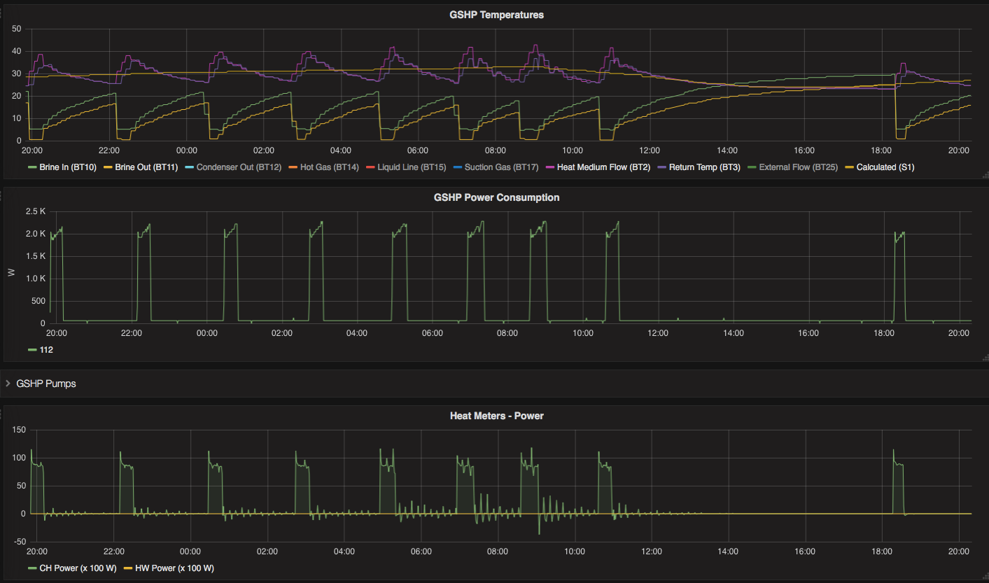
GSHP Performance Graphs for a cold but bright day in February

The second set of graphs (below) show a ‘hot water’ cycle starting at around 2018-02-15T05:00. Note how the increased water delivery temperature (peaking at 55 degrees) corresponds to an increased electricity consumption (peaking at 2.88 kW) while the power output remains steady at 8.0 kW.

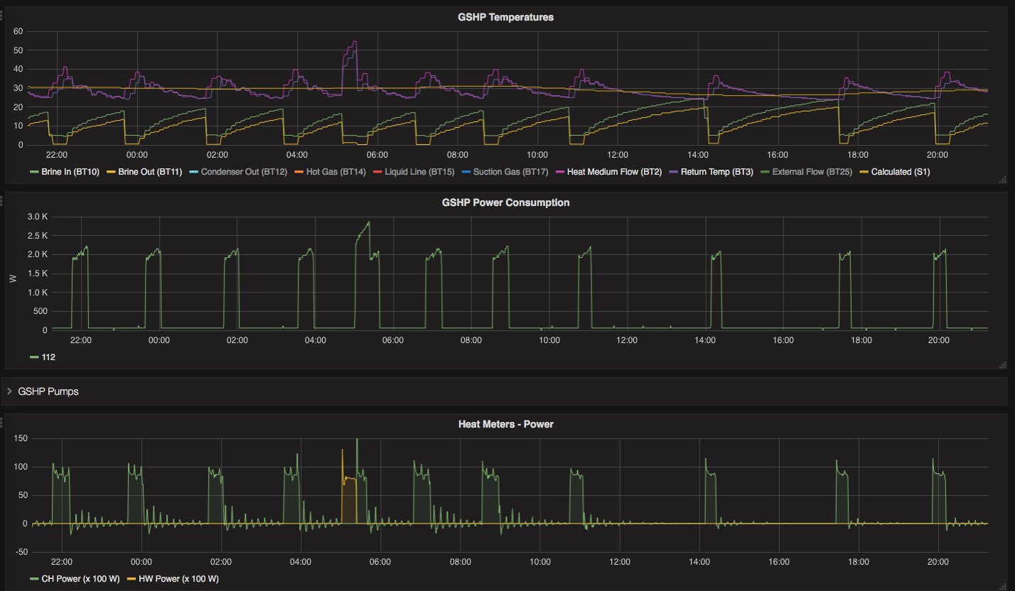
GSHP Performance Graphs for a hot water heating cycle in February

Since I’m the kind of person who likes to measure things “because I can”, it seemed sensible to include Heat Meters on the outputs from the NIBE F1145 Ground Source Heat Pump and also to include an Electrical Sub-Meter on the input. Doing this makes it possible to compare the output power with the input power and calculate the real-world Coefficient of Performance (CoP) of the Heat Pump – a bit like recording all the fuel you put in your car so you can calculate its actual MPG.

The Heat Meters are Kamstrup Multical 302 units with wired M-Bus interfaces which are automatically read every 2 minutes as described in this Technical Article page. Data is published via MQTT and loaded into an InfluxDB database where it can easily be plotted using Grafana.

Two separate Heat Meters are required because there are two separate output pipes from the GSHP – one for the Central Heating and one for the Hot Water. (Within the GSHP unit there’s only a single heat source but there’s a diverter valve that sends water to the appropriate output pipe; the return pipe connection is shared.) While the downside is the cost of the extra heat meter, it does make it easy to see when the heat pump is in ‘heating’ mode versus ‘hot water’ mode – which is important.

The results are quite interesting and reinforce the basic physics of the heat pump operating principles. In summary, the data for my NIBE F1145 shows:

• In ‘heating’ mode, the unit is delivering an instantaneous CoP of as much as 5
• In ‘hot water’ mode, the unit is delivering an instantaneous CoP of as little as 3

Read on for further detail on how these numbers were derived.

Note that at this time of year the ground is still relatively warm and the ‘brine’ coming in from the ground loop is around 10 degrees, returning at around 5 degrees.

Heating

In ‘heating’ mode, the heat pump is configured to deliver water just hot enough to compensate for the heat loss from the house at a given outside temperature. For example, at 4 degrees outside it calculates it wants water at 31 degrees but since the F1145 does not have such a low setting it actually generates water at about 37 degrees. (However it measures how much it is over-delivering by keeping track of the ‘degree minutes’ of the water it produces and won’t turn on again until the average delivery matches its calculated target.) Producing water at 37 degrees, the heat meter records a power output of almost exactly 10 kW while consuming almost exactly 2 kW, giving a CoP of almost exactly 5.

Note that this is an ‘instantaneous’ figure and doesn’t take account of the ongoing low consumption of the GSHP when the compressor isn’t running (consistently showing as 60 W even with the circulation pump running at 30%). Note too that as the weather gets colder outside the water temperature required will increase and the CoP will tend to reduce.

Hot Water

In ‘hot water’ mode, the heat pump is configured to bring the stored hot water up to 50 degrees (except when running the special anti-legionella sterilization cycle where it goes to 60 degrees instead). To do this, it produces water at up to 55 degrees and when doing so the heat meter records a power output of 8.8 kW while consuming up to 2.85 kW – i.e. with a CoP of 3.09.

The ‘up to’ is because the heat pump ramps up its output temperature as the hot water tank heats up, so when the tank is only at 40 degrees the heat pump only bothers delivering water at 45 degrees where it has a much better CoP of around 4.5.

Summary

Overall, the conclusion is that the NIBE F1145 is performing in accordance with its (excellent) published performance figures and has been installed and commissioned well (kudos to Carbon Legacy for that). It’s significantly beating mains gas on both cost and CO2 emissions grounds.

Update 2018-02-16

As the winter has progressed and the ground temperature has reduced the efficiency figures are less impressive than they originally were. See here for a revised set of figures from February rather than November.