The main criterion for Passivhaus-level performance is achieving a space heating requirement better than 15 kWh per m2 of floor area per year (see e.g. this page from the Passivhaus Institut) when heating to an internal temperature of 20C.
One benefit of having a heating system listed on the Heatpump Monitor website is the Heatpump + Fabric dashboard, which orders systems by kWh/m2 and thus provides a direct view of whether buildings are performing at this level.
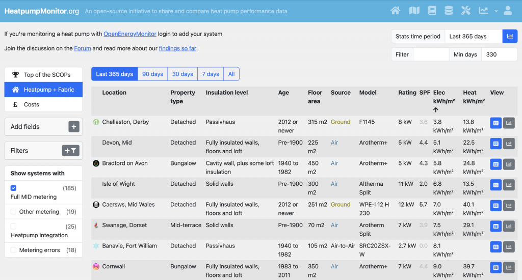
A few points to note:
- By default, this list is sorted by Electricity Input (Elec kWh/m2) rather than Heat Output (Heat kWh/m2) but that’s easy to change.
- It’s not obvious but the Elec and Heat figures relate to the Combined performance of the heat pump, when delivering Space Heating and also when heating Domestic Hot Water.
- There is no indication of the internal temperature achieved, so some buildings might be hotter (or cooler) than the nominal 20C used for the Passivhaus assessment.
The second point tends to increase the consumption figure – potentially quite significantly, because high-performance buildings can use just as much DHW as low-performance buildings, and the higher temperatures required for stored hot water (compared with space heating) results in lower efficiency from a heat pump.
Some systems listed on heatpumpmonitor.org provide additional data on whether they are delivering Space Heating or Hot Water at a particular point in time. If this is accurate, it allows the Hot Water heating periods to be filtered out from the results, providing a more representative view of the heat required for Space Heating. However, it’s clear that many systems don’t accurately report Space Heating mode – so the overall list is unrepresentative. It can be useful to filter out Hot Water production for a single system where the data is known to be accurate.
In my case, looking only at Space Heating drops the kWh / m2 from 13.8 to 13.1, demonstrating that this is even more compliant with the 15.0 kWh / m2 Passivhaus limit (even though the target indoor temperature is 21C, rather than 20C).